Slovenija ima relativno veliko hidro elektrarn, nekaj večjih pa smo na spodnji Savi zgradili tudi v zadnjih letih. Koliko stane taka elektrarna?

Na spodnji Savi smo zgradili pet elektrarn, šesta je še v gradnji. Prva je bila zgrajena že leta 1993, in sicer HE Anhovo. Ostale so precej novejše, in sicer so bile zgrajene po letu 2000. To pomeni, da je dostopnih precej javnih virov, da se lahko ovrednoti stroške gradnje na enoto električne moči. HE Anhovo v tej tabeli ne primerjam, ker je bila zgrajena že tako dolgo nazaj, da za njo nisem našel vrednosti projekta, pa tudi sicer spada pod Savske elektrarne Ljubljana (SEL), medtem ko preostale, ki so spodaj v tabeli, sodijo pod podjetje Hidroelektrarne na spodnji Savi (HE-SS).

Izračun je zelo poenostavljen in sicer samo gledam koliko stane začetna investicija v hidroelektrarno. V energetski del spadajo jez, turbina, generator in generatorska stavba. Za dane elektrarne na kilovat inštalirane moči ta znaša približno 2.400 EUR/kW instalirane moči pri nazadnje zgrajenih hidroelektrarnah pri nas. Seveda v to ni vključeno še vzdrževanje in drugi obratovalni stroški.

Ta velikostni razred je neka približna ocena koliko stane elektrarna take velikosti. Vse te elektrarne imajo po 3 agregate, imajo skupno moč med 30MW in 40MW, večina pa ima projektiran faktor izkoriščenosti okrog 40%. Tako lahko večino časa varno obratuje tudi kadar je en agregat oz. turbina v remontu, kar pa se praviloma izvaja v času nižjih pretokov reke.

Če so stroški za izgradnjo energetskega dela dokaj podobni, so stroški za izgradnjo infrastrukturnega dela precej različni med posamičnimi elektrarnami. Pod infrastrukturni del se šteje ureditev vodotoka, izgradnja nadomestnih cest, izgradnja nasipov in podobno, vse kar je potrebno, da se lahko gorvodno od jezu pojavi zajezitveno jezero, brez da bi to bistveno vplivalo na življenje lokalnih prebivalcev - no, vsaj ljudi. Višina teh stroškov je zelo odvisna od lokacije hidroelektrarne in koliko ter kako obsežni posegi so potrebni.

Infrastrukturni del običajno financira država in lokalna skupnost, energetski del pa energetska družba, ki ima koncesijo za izkoriščanje energije vodnega padca, v tem primeru Hidroelektrarne na spodnji Savi, HESS d.o.o.

HE	Letna proizvodnja (GWh)	Inštalirana moč (MW)	Začetek obratovanja	Faktor izkoriščenosti	Cena izgradnje (infrastrukturni del)	Cena izgradnje (energetski del)	EUR na kW moči
Boštanj	109	32,5	2006	38.3%	26,9 mio	66.976.651 EUR	2061 EUR/kW
Blanca	148	39,12	2009	43.2%	45 mio	92.635.530 EUR	2368 EUR/kW
Krško	146	39,12	2012	42.6%	70,6 mio	95.262.114 EUR	2435 EUR/kW
Brežice	161	47,4	2015	38.8%	141 mio	113 mio EUR	2384 EUR/kW
Mokrice (projektirana)	135	30,5	?	50.5%?	70 mio	100 mio EUR?	3279 EUR/kW?

Viri:

• https://www.hse.si/sl/podpisana-pogodba-o-izvedbi-pripravljalnih-del-za-he-bostanj/
• https://old.delo.si/novice/slovenija/za-gradnjo-he-brezice-ni-dovolj-denarja.html
• Gradnja HE na spodnji Savi: Otvoritev HE Krško - Gradivo za novinarje - HE-SS
• https://old.delo.si/novice/slovenija/zacetek-poskusnega-obratovanja-he-blanca.html
• https://www.dolenjskilist.si/2020/11/06/243677/novice/posavje/Barbic_Gradnja_HE_Mokrice_morda_ze_prihodnje_leto/
• https://www.delo.si/novice/slovenija/politicno-kupckanje-na-srednji-savi/
• https://www.posavskiobzornik.si/gospodarstvo/premier-cerar-ob-odprtju-he-brezice-gre-za-enega-vecjih-projektov-v-eu

Slovenija si je za leto 2020 zadala cilj, da bo pri pridobila četrtino oz. 25 odstotkov končne rabe energije iz obnovljivih virov. Slovenija ima relativno velik delež hidroelektrarn, ki spadajo v obnovljive vire energije, ampak končno rabo obsega tudi neposredna raba energentov npr. za prevoz, ne samo električna energija. Kljub visokemu deležu hidroelektrarn je zadnja leta kazalo, da nam ne bo uspelo, saj so bili skupni deleži obnovljivih virov leta 2017 21,66%, leta 2018 21,38% in leta 2019 21,97%. Premalo.

Lani je sicer k zmanjšani rabi fosilnih goriv pomagal kovidni zaklep družbe, ko je bilo osebnega prometa zelo malo, tako da prve ocene kažejo, da bo delež obnovljivih virov višji, in sicer okrog 23,5%.

Za izpolnitev obljube 25 odstotkov bo morala Slovenija opraviti t.i. čezmejni statistični prenos obnovljivih virov energije. To pomeni, da Slovenija eni drugi državi članici EU plača nekaj denarja, da lahko k svoji kvoti prišteje nekaj njenih megavatnih ur porabljene energije iz obnovljivih virov in si tako lahko čestita, da je dosegla cilje za rabo energije iz obnovljivih virov.

Koliko energije nam umanjka?

Za leto 2020 še ni končnega statističnega poročila koliko energije smo porabili, a če sklepamo po preteklih letih, je končna poraba približno 73% oskrbe s primarnimi energenti. Leta 2020 smo se oskrbeli z 74.647 gigavatnimi urami energije, 73% te vrednosti pa znese 54.489 GWh. Odstotek in pol ocene porabljene energije je 817 GWh.

Cena za statistično preneseno megavatno uro naj bi bila nekje med 12 in 13 euri, kar znese med 9,8 in 10,6 milijona, torej približno 10 milijonov.

Če bi v letu 2020 ne bilo koronskega zaklepa družbe in bi bila oskrba in poraba energije podobna preteklim letom, bi za dokup razlike potrebovali več kot 20 milijonov evrov.

Dopolnitev, 29. november 2021.

Žurnal24 poroča, da smo dosegli 24,16% delež OVE v bruto končni rabi energije. Manjkajoči del do 25%, 455GWh, smo odkupili od Češke za približno 5 milijonov, kar pomeni ceno okrog 11 eurov za megavatno uro.

Opombe, viri in reference:

• Novica o pogajanjih za odkup manjkajočega deleža OVE na energetika.net
• Energetska bilanca, Podatkovna baza SiStat
• Zakon o spodbujanju rabe obnovljivih virov energije, PISRS
• Zgradili premalo sončnih elektrarn, zato bomo pet milijonov evrov plačali Čehom, novica na Žurnal24.si

This friday, a member of the local programmers group on FB put up a question of how the others would approach the problem of finding all valid words from a word list, that can be composed from a list of characters, where letters can repeat. So if you have letters "ABOTOG", you can assemble words TAG, TAB, BOOT, BOAT, etc. This is essentially the same as seen in the Countdown TV game show.

The original poster had already resolved that problem for an online game project, but was curious how others would approach the problem. It sparked a bit of interest in the office and after some debate I set off to see how can this be done in Postgres.

Setup

I found a word list of 370.000 english words to test how the queries perform (words_alpha.txt from a github repo). This is how I created the table and imported the data:

 create table wordlist (word text);
 \copy wordlist from 'words_alpha.txt';
 select count(*) from wordlist ;
  count
---------
  370099
 (1 row)

Original author's SQL query

The author's original query was a MySQL version of this query:

SELECT word FROM wordlist WHERE
char_length(word)-char_length(replace(upper(word),'A','')) <= 0
AND char_length(word)-char_length(replace(upper(word),'B','')) <= 0
AND char_length(word)-char_length(replace(upper(word),'C','')) <= 0
AND char_length(word)-char_length(replace(upper(word),'D','')) <= 0
AND char_length(word)-char_length(replace(upper(word),'E','')) <= 2
AND char_length(word)-char_length(replace(upper(word),'F','')) <= 0
AND char_length(word)-char_length(replace(upper(word),'G','')) <= 1
AND char_length(word)-char_length(replace(upper(word),'H','')) <= 0
AND char_length(word)-char_length(replace(upper(word),'I','')) <= 1
AND char_length(word)-char_length(replace(upper(word),'J','')) <= 1
AND char_length(word)-char_length(replace(upper(word),'K','')) <= 0
AND char_length(word)-char_length(replace(upper(word),'L','')) <= 0
AND char_length(word)-char_length(replace(upper(word),'M','')) <= 1
AND char_length(word)-char_length(replace(upper(word),'N','')) <= 1
AND char_length(word)-char_length(replace(upper(word),'O','')) <= 0
AND char_length(word)-char_length(replace(upper(word),'P','')) <= 0
AND char_length(word)-char_length(replace(upper(word),'R','')) <= 0
AND char_length(word)-char_length(replace(upper(word),'S','')) <= 0
AND char_length(word)-char_length(replace(upper(word),'T','')) <= 0
AND char_length(word)-char_length(replace(upper(word),'U','')) <= 1
AND char_length(word)-char_length(replace(upper(word),'V','')) <= 0
AND char_length(word)-char_length(replace(upper(word),'Z','')) <= 0
AND char_length(word)-char_length(replace(upper(word),'X','')) <= 0
AND char_length(word)-char_length(replace(upper(word),'Y','')) <= 0
AND char_length(word)-char_length(replace(upper(word),'Q','')) <= 0
AND char_length(word)-char_length(replace(upper(word),'W','')) <= 0;

This compares the letter count in the words and is relatively easy to understand, but is somewhat resource intensive. This was the query plan Postgres took:

                                                QUERY PLAN
--------------------------------------------------------------------------------------------------------------------
 Seq Scan on public.wordlist  (cost=0.00..149953.60 rows=1 width=10) (actual time=113.228..755.601 rows=120 loops=1)
   Output: word
   Filter: (((char_length(wordlist.word) - char_length(replace(upper(wordlist.word), 'A'::text, ''::text))) <= 0) AND ((char_length(wordlist.word) - char_length(replace(upper(wordlist.word)
   Rows Removed by Filter: 369979
   Buffers: shared hit=1914
 Planning time: 0.273 ms
 Execution time: 755.696 ms
(7 rows)

Regex queries

The easiest win is using regex in a query. With it you can limit which letters may be used in a word, and it works surprisingly well, essentially doing a sequential scan, reading full table and seeing if words match. This is the query for the letters "EJIGUNEM":

explain (analyze, verbose, buffers) select word from wordlist where word ~* '^[EJIGUNEM]+$';
                                                QUERY PLAN
--------------------------------------------------------------------------------------------------------------------
 Seq Scan on public.wordlist  (cost=0.00..6540.24 rows=37 width=10) (actual time=40.506..142.450 rows=249 loops=1)
   Output: word
   Filter: (wordlist.word ~* '^[EJIGUNEM]+$'::text)
   Rows Removed by Filter: 369850
   Buffers: shared hit=1914
 Planning time: 0.220 ms
 Execution time: 142.491 ms
(7 rows)

A trained eye will spot that a regex does not actually enforce letter repetition limit and therefore returns 249 rows instead of correct 120. Since I was doing this before the original author posted his solution, I created a python function which checks if a word can be composed from given chars, but you could equally well use his query to filter the words:

create or replace function can_word(word text, chars text) returns boolean
language plpython3u immutable strict as $f$
valid_chars = [c for c in chars.lower()]
for c in word:
    try:
        valid_chars.remove(c)
    except:
        return False
return True
$f$;

With this extra check the query then becomes:

 explain (analyze, verbose, buffers)
 with words_maybe as (select word from wordlist where word ~* '^[EJIGUNEM]+$')
 select word from words_maybe where can_word(word, 'EJIGUNEM');
                                                         QUERY PLAN
----------------------------------------------------------------------------------------------------------------------------
  CTE Scan on words_maybe  (cost=6540.24..6550.23 rows=12 width=32) (actual time=42.183..150.407 rows=120 loops=1)
    Output: words_maybe.word
    Filter: can_word(words_maybe.word, 'EJIGUNEM'::text)
    Rows Removed by Filter: 129
    Buffers: shared hit=1914
    CTE words_maybe
      ->  Seq Scan on public.wordlist  (cost=0.00..6540.24 rows=37 width=10) (actual time=42.141..148.823 rows=249 loops=1)
            Output: wordlist.word
            Filter: (wordlist.word ~* '^[EJIGUNEM]+$'::text)
            Rows Removed by Filter: 369850
            Buffers: shared hit=1914
  Planning time: 0.190 ms
  Execution time: 150.443 ms
 (13 rows)

This query returns the correct 120 rows and it works in a decent enough time for most developers to stop here.

Cube extension

If we can represent letters as a vector, we could try the cube extension. Let's create a function that evolves the original author's query and creates a full vector from the letter count (we're assuming the alphabet is ASCII letters only here):

create or replace function word2vec(word text) returns cube
language plpython3u immutable strict as $f$
cu = [0] * 26

for c in word.upper():
    intc = ord(c)
    if 65 <= intc <= 90:
        cu[(intc - 65)] += 1
    else:
        return None
return str(tuple(cu))
$f$;

We can now create an index over the letter vectors, but we also include word in the index, in order to enable postgres to return word while only accessing index and not touching the heap:

create index wordlist_word_vec on wordlist using gist (word2vec(word), word);

And query is now magically fast:

 explain (analyze, verbose, buffers) select word from wordlist where word2vec(word) <@ cube_union(word2vec('EJIGUNEM'), '0');
                                                                                                        QUERY PLAN
-------------------------------------------------------------------------------------------------------------------------------------------------------------------------------------------------------------------------
  Bitmap Heap Scan on public.wordlist  (cost=95.28..1118.29 rows=370 width=10) (actual time=7.518..7.650 rows=120 loops=1)
    Output: word
    Recheck Cond: (word2vec(wordlist.word) <@ '(0, 0, 0, 0, 0, 0, 0, 0, 0, 0, 0, 0, 0, 0, 0, 0, 0, 0, 0, 0, 0, 0, 0, 0, 0, 0),(0, 0, 0, 0, 2, 0, 1, 0, 1, 1, 0, 0, 1, 1, 0, 0, 0, 0, 0, 0, 1, 0, 0, 0, 0, 0)'::cube)
    Heap Blocks: exact=67
    Buffers: shared hit=1737
    ->  Bitmap Index Scan on wordlist_word_vec  (cost=0.00..95.18 rows=370 width=0) (actual time=7.500..7.500 rows=120 loops=1)
          Index Cond: (word2vec(wordlist.word) <@ '(0, 0, 0, 0, 0, 0, 0, 0, 0, 0, 0, 0, 0, 0, 0, 0, 0, 0, 0, 0, 0, 0, 0, 0, 0, 0),(0, 0, 0, 0, 2, 0, 1, 0, 1, 1, 0, 0, 1, 1, 0, 0, 0, 0, 0, 0, 1, 0, 0, 0, 0, 0)'::cube)
          Buffers: shared hit=1670
  Planning time: 0.370 ms
  Execution time: 7.726 ms
 (10 rows)

Queries are now fast, using index and returning 120 matching rows in sub 10ms. While the original table is only 15MB, the index is much bigger at 176MB, so it's a common memory vs. CPU time tradeoff.

Every now and then a sysadmin or a developer comes into a situation where he wishes he had not created one big partition or deletes a partition and wishes to grow one file system over the next partition. Besides growing file system, btrfs also supports shrinking in a seemingly simple command. Because the filesystem and partition meddling is always a scary operation, I was wondering if the resize operation actually moves data on btrfs.

This simple test uses blktrace and seekwatcher to trace and visualize how has the file system actually been accessing the underlying block device.

For the test, I'm using kernel 4.9.20 and btrfs-progs 4.7.3.

/btrfs-test# dd if=/dev/zero of=btrfs.img bs=1M count=2048
2048+0 records in
2048+0 records out
2147483648 bytes (2.1 GB, 2.0 GiB) copied, 4.6457 s, 462 MB/s

/btrfs-test# losetup -f btrfs.img
/btrfs-test# losetup -a
/dev/loop0: [2051]:538617527 (/btrfs-test/btrfs.img)

/btrfs-test# mkfs.btrfs --mixed /dev/loop0
btrfs-progs v4.7.3
See http://btrfs.wiki.kernel.org for more information.

Performing full device TRIM (2.00GiB) ...
Label:              (null)
UUID:
Node size:          4096
Sector size:        4096
Filesystem size:    2.00GiB
Block group profiles:
  Data+Metadata:    single            8.00MiB
  System:           single            4.00MiB
SSD detected:       no
Incompat features:  mixed-bg, extref, skinny-metadata
Number of devices:  1
Devices:
   ID        SIZE  PATH
    1     2.00GiB  /dev/loop0

#!/bin/bash

cp -v ubuntu-16.04.2-server-amd64.iso testmnt/server-iso1.iso
cp -v ubuntu-16.04.2-server-amd64.iso testmnt/server-iso2.iso

sync
sleep 3

cp -v mini.iso testmnt/mini.iso

sync
sleep 6

rm testmnt/server-iso*
sync
sleep 3

btrfs filesystem resize 1G testmnt/
sync

/btrfs-test# blktrace -d /dev/loop0 -o trace1
^C=== loop0 ===
  CPU  0:                19029 events,      892 KiB data
  CPU  1:                27727 events,     1300 KiB data
  CPU  2:                28491 events,     1336 KiB data
  CPU  3:                28879 events,     1354 KiB data
  Total:                104126 events (dropped 0),     4881 KiB data

/btrfs-test$ seekwatcher -t trace1.blktrace
using tracefile ././trace1
saving graph to trace.png

Test results

The following graph shows how the at the start of script (first 5 seconds) most of the disk is filled, when the two copies of ubuntu are placed on the drive. Then at 16 seconds, the mini.iso is placed almost at the end of drive. At about 26 seconds the resize operation is done, where the filesystem does actually move the mini.iso to another place on device. Yay!

Full seekwatcher graph

Besides disk offset, seekwatcher also displays throughput, seek count and IOPs, all nicely aligned by time so you can quickly see what is happening with disks when you need to, as seen in the whole graph below.

I've been playing a bit with BTRFS lately. The file system has checksums of both metadata and data so it can offer some guarantees about data integrity and I decided to take a closer look at it hoping I could see if it can keep any of the data that we people try keep on our unstable hardware.

# losetup -f 2017-03-02-raspbian-jessie-lite.img
# losetup -a
/dev/loop0: [2051]:203934014 (/home/user/rpi-image-build/2017-03-02-raspbian-jessie-lite.img)
# kpartx -av /dev/loop0
add map loop0p1 (254:0): 0 129024 linear 7:0 8192
add map loop0p2 (254:1): 0 2584576 linear 7:0 137216
# mkdir rpi_root
# mount /dev/mapper/loop0p2 rpi_root
# (cd rpi_root && tar zcf ../root.tar.gz . && find . -type f -exec sha1sum {} \; > ../sha1sums)
# umount rpi_root
# kpartx -dv /dev/loop0
del devmap : loop0p2
del devmap : loop0p1
# losetup -d /dev/loop0

#!/usr/bin/python
import os
import random

f = 'rpi-btrfs-test.img'
fd = open(f, 'rb+')
filesize = os.path.getsize(f)

print('filesize=%d' % filesize)
random_data = str(bytearray([random.randint(0, 255) for i in range(4096)]))

count = 0
loopcount = 0
while count < 100:
    n = random.randint(0, filesize/4096)
    fd.seek(n*4096)
    block = fd.read(4096)

    if any((i != '\x00' for i in block)):
        print('corrupting block %d' % n)

        fd.seek(n*4096)
        fd.write(random_data)

        assert fd.tell() == (n+1)*4096
        count += 1

    loopcount += 1
    if loopcount > 10000:
        break
fd.close()

dd if=/dev/zero of=rpi-btrfs-test.img bs=1M count=4096

# mkfs.ext4 -O metadata_csum,64bit rpi-btrfs-test.img
mke2fs 1.43.4 (31-Jan-2017)
Discarding device blocks: done
Creating filesystem with 1048576 4k blocks and 262144 inodes
Filesystem UUID: c8c7b1cc-aebc-44a3-bb6d-790fb3b70577
Superblock backups stored on blocks:
        32768, 98304, 163840, 229376, 294912, 819200, 884736

Allocating group tables: done
Writing inode tables: done
Creating journal (16384 blocks): done
Writing superblocks and filesystem accounting information: done

mkdir mnt
mount -o loop rpi-btrfs-test.img mnt
(cd mnt && tar zxf ../root.tar.gz)

# df -h
/dev/loop0      3.9G  757M  3.0G  21% /home/user/rpi-image-build/mnt

umount mnt
python corrupt.py

 # fsck.ext4 -y -v -f rpi-btrfs-test.img
 e2fsck 1.43.4 (31-Jan-2017)
 Pass 1: Checking inodes, blocks, and sizes
 Pass 2: Checking directory structure
 Directory inode 673, block #0, offset 0: directory has no checksum.
 Fix? yes

 ... lots of prinouts of error and repair info

 Pass 5: Checking group summary information

 rpi-btrfs-test.img: ***** FILE SYSTEM WAS MODIFIED *****

        35610 inodes used (13.58%, out of 262144)
           65 non-contiguous files (0.2%)
            7 non-contiguous directories (0.0%)
              # of inodes with ind/dind/tind blocks: 0/0/0
              Extent depth histogram: 30289/1
       226530 blocks used (21.60%, out of 1048576)
            0 bad blocks
            1 large file

        27104 regular files
         3038 directories
           54 character device files
           25 block device files
            0 fifos
          346 links
         5380 symbolic links (5233 fast symbolic links)
            0 sockets
-------------
        35946 files

mount -o loop rpi-btrfs-test.img mnt

# (cd mnt && sha1sum -c ../sha1sums | grep -v 'OK' )

... lots of files with FAILED

./usr/lib/arm-linux-gnueabihf/libicudata.so.52.1: FAILED
sha1sum: WARNING: 1 listed file could not be read
sha1sum: WARNING: 90 computed checksums did NOT match

# mkfs.btrfs --mixed rpi-btrfs-test.img
btrfs-progs v4.7.3
See http://btrfs.wiki.kernel.org for more information.

Label:              (null)
UUID:
Node size:          4096
Sector size:        4096
Filesystem size:    4.00GiB
Block group profiles:
  Data+Metadata:    single            8.00MiB
  System:           single            4.00MiB
SSD detected:       no
Incompat features:  mixed-bg, extref, skinny-metadata
Number of devices:  1
Devices:
   ID        SIZE  PATH
    1     4.00GiB  rpi-btrfs-test.img

mount -o loop rpi-btrfs-test.img mnt
(cd mnt && tar zxf ../root.tar.gz)

# df -h
/dev/loop0      4.0G  737M  3.3G  18% /home/user/rpi-image-build/mnt

umount mnt
python corrupt.py

# mount -o loop rpi-btrfs-test.img mnt
# btrfs scrub start mnt/
scrub started on mnt/, fsid a6301050-0d88-4d86-948d-03380b9434d4 (pid=27478)
# btrfs scrub status mnt/
scrub status for a6301050-0d88-4d86-948d-03380b9434d4
    scrub started at Sun Apr 30 10:17:12 2017 and was aborted after 00:00:00
    total bytes scrubbed: 272.49MiB with 37 errors
    error details: csum=37
    corrected errors: 0, uncorrectable errors: 37, unverified errors: 0

# (cd mnt && sha1sum -c ../sha1sums | grep -v 'OK' )
sha1sum: ./usr/share/perl5/Algorithm/Diff.pm: Input/output error
./usr/share/perl5/Algorithm/Diff.pm: FAILED open or read

... lots more of terminal output similar to above

sha1sum: WARNING: 99 listed files could not be read

# mkfs.btrfs --data dup --metadata dup --mixed rpi-btrfs-test.img
btrfs-progs v4.7.3
See http://btrfs.wiki.kernel.org for more information.

Label:              (null)
UUID:
Node size:          4096
Sector size:        4096
Filesystem size:    4.00GiB
Block group profiles:
  Data+Metadata:    DUP             204.75MiB
  System:           DUP               8.00MiB
SSD detected:       no
Incompat features:  mixed-bg, extref, skinny-metadata
Number of devices:  1
Devices:
   ID        SIZE  PATH
    1     4.00GiB  rpi-btrfs-test.img

mount -o loop rpi-btrfs-test.img mnt
(cd mnt && tar zxf ../root.tar.gz)

# df -h | grep mnt
/dev/loop0      2.0G  737M  1.3G  36% /home/user/rpi-image-build/mnt

umount mnt
python corrupt.py

# mount -o loop rpi-btrfs-test.img mnt
# btrfs scrub start mnt/
scrub started on mnt/, fsid 12ffd7a2-b9c4-46ca-b16a-cd07d94d6854 (pid=27863)
# btrfs scrub status mnt/
scrub status for 12ffd7a2-b9c4-46ca-b16a-cd07d94d6854
    scrub started at Sun Apr 30 10:27:31 2017 and finished after 00:00:00
    total bytes scrubbed: 1.41GiB with 99 errors
    error details: csum=99
    corrected errors: 99, uncorrectable errors: 0, unverified errors: 0

# (cd mnt && sha1sum -c ../sha1sums | grep -v 'OK' )

Did you know KVM has a way to enable discard pass thru? I did, but then I forgot and had to google again.

This is how you do it:

kvm -drive discard=unmap,file=debian.qcow2,id=ff,if=none \
    -device virtio-scsi-pci -device scsi-disk,drive=ff

When booted, you have to make sure your fs is mounted with discard option, and can then do:

fstrim /

And the image on the host should be significantly smaller. Use du or ls -alsh, not just ls, because ls does not display actual disk usage if you don't pass -s:

1,4G -rw-r--r--  1 root root 4,0G apr  7 17:22 debian.img

Now you know.

Did you know you can start kvm with vnc disabled and then attach it in monitor? And change CD or save vm snapshot?

"Moving objects" or "spatio-temporal database" is a database, which stores data with temporal and spatial aspects. One example is keeping a database of how real estate changes through time, another a bit more interactive is, say, tracking location and movement of vehicles through time and keeping the history in database.

What we want to be able to answer is such questions as:

• where have the tracked objects been over time,
• check whether an tracked object has passed through a checkpoint,
• check if two tracked objects have crossed paths,
• if two tracked objects have crossed paths, where and at what time has this happened?

To achieve this, we will combine two PostgreSQL's features: builtin range data types and operators, and spatial data types and operators provided by PostGIS extension.

For the example here, we will use GPX track exports of some of my runs. First we need to import GPX data into a table we create:

CREATE TABLE gpx (
    id integer,
    filename text,
    lat numeric,
    lon numeric,
    ts timestamptz);

I created a small Python script converter.py, which reads GPX XMLs in current dir and outputs CSV with coordinates out stdout. This is then directly usable in psql's \COPY command:

\COPY gpx FROM PROGRAM 'python converter.py' WITH CSV;

COPY 17549
Time: 617,839 ms

Modeling spatial aspects

Postgres supports spatial data types via PostGIS extension. I will not go into full detail about PostGIS here, for now it suffices to know it works by adding a geometry column to our table and that it allows us to index this column, which enables fast lookups. In my example we will model the distance the object covered with line geometry. Besides linestrings (lines), there are also points and polygons.

Modeling temporal aspects

Postgres supports ranged types, and among them are also time ranges. daterange is a range between two dates and tstzrange is a range between two timestamptz values. Ranges in Postgres are canonically represented in included-excluded notation, meaning the start of the range is included and the end of the range is excluded but marks the boundary and all values less than that are included. Example:

 SELECT '[2016-01-01, 2016-06-30]'::daterange;
         daterange
---------------------------
  [2016-01-01,2016-07-01)
 (1 row)

With this, we created a date range for the first half of this year, that is between first of January inclusive and last of June inclusive. We can see Postgres normalizes this into 1st January inclusive and 1st July exclusive.

A table for tracking objects

For tracking objects, lets create a new table. Table needs to have a few fields: a serial for identifying each segment, an object identifier to know which object the time and location belongs to, and, of course, time period and corresponding location of the object:

CREATE TABLE tracks (
    id serial,
    object_id integer,
    timeslice tstzrange);

You will notice the location is missing! The geometry columns are added via a special function AddGeometryColumn. We need to provide a number of parameters. Table name and column name are obvious. Next we need to provide spatial reference ID, which uniquely identifies a number of parameters required for correctly interpreting spatial data - here we use ID 4326, which denotes the WGS84 world geodetic system. Geometry type we'll be using is LINESTRING and the last parameter is number of dimensions, which is two:

SELECT AddGeometryColumn('tracks', 'geom', 4326, 'LINESTRING', 2);

Now we want to convert GPX data into tracks. Tracks will have temporal intervals in field timeslice and lines in field geom.

With following query we can convert numerical values in table gpx to real point data type. We use ST_MakePoint to create a point and ST_SetSRID, to set spatial reference system on geometry so PostGIS knows how to interpret it:

--- example
SELECT id, ts, ST_SetSRID(ST_MakePoint(lon, lat), 4326) pt FROM gpx;

Having points, we can use "lead" window function to pair current timestamp and point with timestamp and point in the next row:

--- example
SELECT
    id,
    ts,
    lead(ts) OVER (PARTITION BY id ORDER BY ts ASC) next_ts,
    pt,
    lead(pt) OVER (PARTITION BY id ORDER BY ts ASC) next_pt
FROM points;

Having such two timestamps and points in the same row, all we have to do now is join them into ranged types. Here we must be careful to exclude the last row, since the next_pt and next_ts are both NULL and will not generate correct geometry and time range:

--- example
SELECT
    id AS object_id,
    ST_MakeLine(pt, next_pt) geom,
    tstzrange(ts, next_ts) timeslice
FROM twopoints
WHERE next_pt IS NOT NULL ORDER BY id, ts ASC;

Now we can create a pipeline and join above three queries into one using WITH statement and insert resulting data into tracks table:

WITH
    points AS (
        SELECT id, ts, ST_SetSRID(ST_MakePoint(lon, lat), 4326) pt FROM gpx),
    twopoints AS (
        SELECT
            id,
            ts,
            lead(ts) OVER (PARTITION BY id ORDER BY ts ASC) next_ts,
            pt,
            lead(pt) OVER (PARTITION BY id ORDER BY ts ASC) next_pt
        FROM points),
    segments_and_timeslices AS (
        SELECT
            id AS object_id,
            ST_MakeLine(pt, next_pt) geom,
            tstzrange(ts, next_ts) timeslice
        FROM twopoints
        WHERE next_pt IS NOT NULL ORDER BY id, ts ASC)
INSERT INTO tracks (object_id, timeslice, geom)
SELECT object_id, timeslice, geom FROM segments_and_timeslices;

INSERT 0 17543
Time: 413,548 ms

There. In table tracks, we now have all we need to get meaningful results to the questions above. To make it speedy, we need to add a few more indexes:

modb=# CREATE INDEX tracks_timeslice_idx ON tracks USING GIST (timeslice);
CREATE INDEX
Time: 250,054 ms
modb=# CREATE INDEX tracks_geom_idx ON tracks USING GIST (geom);
CREATE INDEX
Time: 96,496 ms

Answering the questions

Now we can check where an object has been on 7th May this year between 13h and 14h. We do this by using && overlap operator with tstzrange:

SELECT
    A.id,
    A.object_id,
    A.geom
FROM tracks A
WHERE
    A.timeslice && '[2016-05-07 13:00:00+02,2016-05-07 14:00:00+02)'::tstzrange
    AND A.object_id = 0;

   id   | object_id |                                            geom
---------+-----------+--------------------------------------------------------------------------------------------
 117576 |         0 | 0102000020E610000002000000D0B4C4CA681C2D40B2D6506A2F044740AE4676A5651C2D40E84B6F7F2E044740
 117577 |         0 | 0102000020E610000002000000AE4676A5651C2D40E84B6F7F2E0447408CD82780621C2D408F34B8AD2D044740
...

Check if any two objects have crossed paths. In geometry, there's also && overlap operator, but it checks if the bounding boxes of compared geometries overlap, not the actual geometries. This is why we have to use another function here, ST_Intersects, which is exact:

SELECT A.object_id, B.object_id, A.id, B.id
FROM tracks A, tracks B
WHERE
    ST_Intersects(A.geom, B.geom)
    AND A.timeslice && B.timeslice
    AND A.id != B.id
    AND A.object_id < B.object_id;

 object_id | object_id | id | id
------------+-----------+----+----
(0 rows)

Time: 1032,741 ms

Obviously, since all the tracks are from me, I can't cross paths with myself. But we can use postgres to time travel one of my runs forward in time exactly the right amount to make it cross another:

UPDATE tracks
SET
    timeslice = tstzrange(
        lower(timeslice) + interval '302 days 20:33:37',
        upper(timeslice) + interval '302 days 20:33:37',
        '[)')
WHERE object_id = 5;

UPDATE 4632
Time: 164,788 ms

And now, if we repeat above query:

SELECT A.object_id, B.object_id, A.id, B.id
FROM tracks A, tracks B
WHERE
    ST_Intersects(A.geom, B.geom)
    AND A.timeslice && B.timeslice
    AND A.id != B.id
    AND A.object_id < B.object_id;

 object_id | object_id |   id   |   id
------------+-----------+--------+--------
         4 |         5 | 129396 | 133243
(1 row)

Time: 1099,215 ms

In this query it is enough to go through half of returned rows, since we are comparing all the tracks with all of the other and including only one permutation is enough. That's why we limit the query with A.object_id < B.object_id.

Checking if an object has passed a checkpoint then means specifying a line denoting checkpoint and looking up intersections with it in tracks table - an exercise left for the reader.

Modeling moving objects with ranges and lines is just one way. Your database representation might vary a lot depending on questions the users will be asking about the data.

Hopefully this tutorial has made a case how ranged data types in postgres can make otherwise very intensive task - finding intersections in both spatial and temporal dimensions - relatively simple.

Prejšnji teden sem bil v Bilbau, na konferenci EuroPython 2016. Na konferenci smo obiskovalci brezplačno dobili mini računalnik BBC micro:bit.

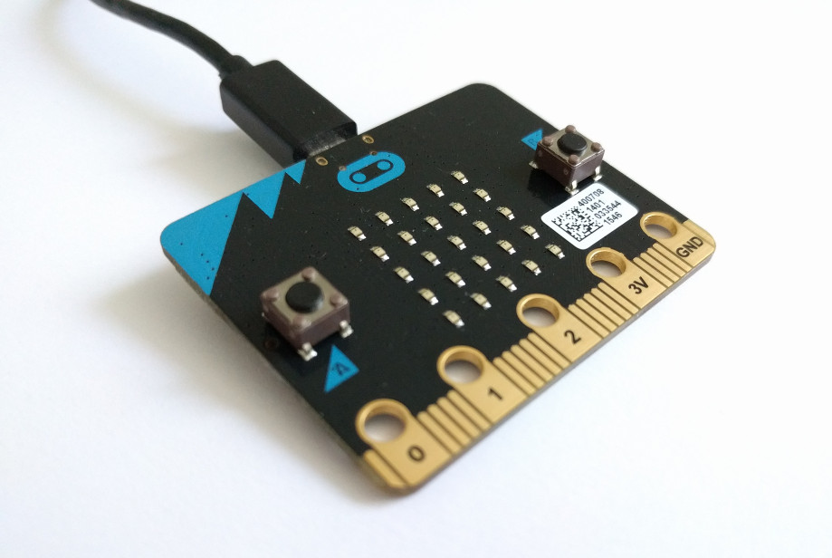
BBC micro:bit je poleg Raspberry Pi še eden izmed mini računalnikov, posebej namenjenih izobraževanju mladih, da se pobliže spoznajo s samim delovanjem računalnikov, ne samo s površnega klikanja z miško in dotikanja s prstom po uporabniških vmesnikih. Spoznajo do te mere, da se naučijo osnov kako računalniki razumejo zelo osnovna navodila, ki jim jih posredujejo ljudje, ter se naučijo računalnike uporabljati kot kreativno orodje, ne zgolj kot (pasivno) sredstvo za konzumacijo (multi-) medijskih vsebin.

Micro:bit je posebej namenjen izobraževanju: na ploščici je poleg procesorja še 25 rdečih LED lučk in dva gumba, s tem pa se da že marsikaj zanimivega naredit. Poleg lučk in gumbov sta še dva senzorja, pospeškomer (akcelerometer) ter magnetometer (kompas), s katerima se da zaznavati orientacijo ploščice ter orientacijo oz. tudi bližino kovine. Ploščica se lahko povezuje z drugimi ploščicami bodisi preko žic, bodisi preko brezžične povezave z uporabo Bluetooth Low Energy.

Zakaj se imenuje BBC micro:bit? Ker je nastala v sodelovanju z BBC v okviru programa digitalne pismenosti, cilj britancev pa je napravo zastonj podarit milijonu otoških osnovnošolcev z željo, da bi se čim več mladih prijelo tudi nekaj računalniškega znanja.

Delo s ploščico je sila enostavno, za delo je dovolj osebni računalnik, ploščica in povezovalni kabel. Za pričetek programiranja je dovolj kar uporaba spletnega urejevalnika, ki je dostopen na microbit.co.uk, čeprav je res, da je (vsaj za Python) tam nekoliko zastarela koda. Spletni urejevalnik omogoča, da kar v brskalniku sprogramiramo željeno funkcionalnost, z gumbom "Download" pa potem prenesemo program, ki ga shranimo na microbit, ki se računalniku predstavi kot USB ključek. Microbit bo to zaznal, naložil program in ga začel izvajat in napravica bo zaživela.

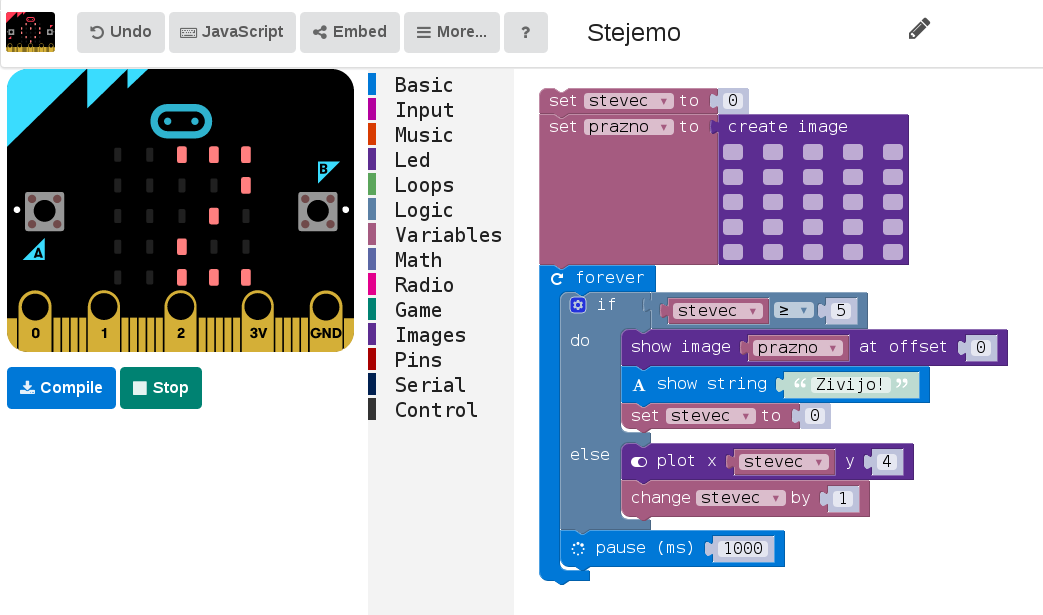
Poleg uradne strani sta na voljo še dva urejevalnika, pri prvem - Code the microbit - se program sestavlja z grafičnimi bloki, ki precej poenostavijo sestavljanje programa. Ponuja tudi "predvajanje" programa, da je takoj vidno delovanje. Programiranje deluje enako, program prenesemo prek spleta in ga odložimo na microbit, ki se osebnemu računalniku predstavi kot USB ključek.

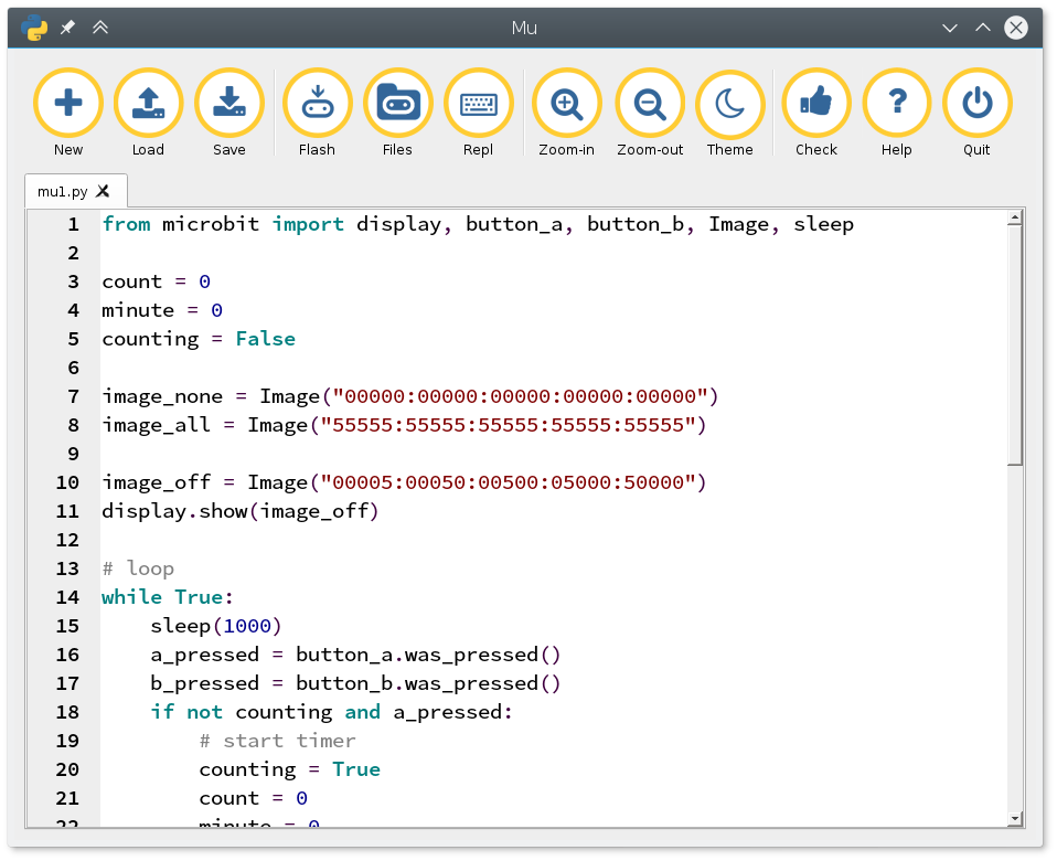
Mu je namenski urejevalnik za MicroPython kodo, ki ga prenesemo in poženemo na osebnem računalniku. Ta omogoča naprednejše programiranje v Pythonu in neposredno zazna microbit, tako da ni potrebno ročno kopirati datotek.

Oba urejevalnika omogočata sestavljanje kompleksnih opravil, ki so zamejena predvsem z domišljijo, tem pa (vsaj otrokom) ne zmanjka. S tako cenovno dostopno napravico - stane približno 15 eur - verjamem, da se da delat zabavne delavnice.

I've previously blogged about colors and PostgreSQL here. In this post I will cover some insight into custom GiST index, which enables efficiently looking up similar colors.

Color distance measures

There are several revisions of Delta E color distance measure, each more accurate and more complicated. The first revision is called CIE 1976. After further research in (human) color perception it became clear the CIE 1976 has deficiencies and revised versions CIE 1994 and later CIE 2000 were released.

Numerically, CIE 1976 is just euclidean, straight line distance between points in L*a*b color space, as this color space was defined such to have this property. The CIE 2000 Delta E is far more complex and non uniform and lacks this property, so we can't use CIE 2000 with vanilla PostgreSQL 9.6.

So let's see how you can implement CIE 1976 color similarity search with PostgreSQL 9.6.

PostgreSQL cube extension

Cube contrib extension is a custom PostgreSQL data type, with which you can represent N-dimensional vectors. It also supports indexes, so you can efficiently look up values based on column of this data type.

Let's load the extension:

colorsdb=# create extension cube;
CREATE EXTENSION

Okay, quick overview how cube works! We can create a sample point and check it is a point:

 colorsdb=# select '(1,2,3)'::cube;
    cube
------------
  (1, 2, 3)
 (1 row)

 colorsdb=# select cube_is_point('(1,2,3)'::cube);
  cube_is_point
----------------
  t
 (1 row)

Or we can create a 3x3x3 cube and check its size:

 colorsdb=# select '(1,2,3),(4,5,6)'::cube;
         cube
----------------------
  (1, 2, 3),(4, 5, 6)
 (1 row)

 colorsdb=# select cube_is_point('(1,2,3),(4,5,6)'::cube);
  cube_is_point
----------------
  f
 (1 row)

 colorsdb=# select cube_size('(1,2,3),(4,5,6)'::cube);
  cube_size
------------
         27
 (1 row)

Cube data type is perfectly suited for color space representation. You can store the colors as 3-dimensional points in space, where point is a special case of cube - it has zero volume and has both upper right and lower left points equal.

You can get euclidean distance with cube_distance:

 colorsdb=# select cube_distance('(1,2,3)'::cube, '(1,2,6)'::cube);
  cube_distance
----------------
              3
 (1 row)

In upcoming PostgreSQL 9.6 version, this extension will also support distance operators. Here, <-> is an euclidean distance operator:

 colorsdb=# select '(1,2,3)'::cube <-> '(1,2,6)'::cube;
  ?column?
-----------
         3
 (1 row)

Let's create an test table with 500.000 records:

create table colors (color cube);

with random_colors as (
    select
        random() * 100 as l,
        random() * 255 - 128 as a,
        random() * 255 - 128 as b
    from generate_series(1, 500000) x)
insert into colors select cube(array[l,a,b]) from random_colors;

And we can now select 5 closest colors to (1,2,3):

colorsdb=# select '(1,2,3)'::cube <-> color, color from colors order by 1 asc limit 5;
     ?column?     |                            color
-------------------+-----------------------------------------------------------
 1.61559798496189 | (1.89253129065037, 1.71048436127603, 1.68480973271653)
 2.55645225973282 | (3.37235750630498, 1.64988295687363, 3.88588152406737)
 2.55950246687413 | (2.91422470472753, 1.19065871741623, 4.493908747565)
 2.85963596867927 | (1.00834178738296, 4.51141274580732, 4.3675724142231)
 3.11127226552722 | (1.72140300273895, 3.04948928579688, 0.161309270653874)
(5 rows)

What is the cost for this:

 colorsdb=# explain analyze select '(1,2,3)'::cube <-> color, color from colors order by 1 asc limit 10;
                                                         QUERY PLAN
----------------------------------------------------------------------------------------------------------------------------
  Limit  (cost=20734.28..20734.30 rows=10 width=40) (actual time=151.844..151.846 rows=10 loops=1)
    ->  Sort  (cost=20734.28..21984.46 rows=500072 width=40) (actual time=151.843..151.845 rows=10 loops=1)
          Sort Key: (('(1, 2, 3)'::cube <-> color))
          Sort Method: top-N heapsort  Memory: 25kB
          ->  Seq Scan on colors  (cost=0.00..9927.90 rows=500072 width=40) (actual time=0.014..88.199 rows=500000 loops=1)
  Planning time: 0.054 ms
  Execution time: 151.864 ms
 (7 rows)

You can see PostgreSQL is doing a sequential scan and it takes 151 ms to get 5 nearest colors. Without index, that is. Since 9.1, PostgreSQL supports returning nearest items with use of GiST index. Let's try indexing colors (building index takes a while):

colorsdb=# create index colors_color_idx on colors using gist (color);
CREATE INDEX

And check the query now:

 colorsdb=# explain analyze select '(1,2,3)'::cube <-> color, color from colors order by 1 asc limit 10;
                                                                 QUERY PLAN
-------------------------------------------------------------------------------------------------------------------------------------------
  Limit  (cost=0.29..1.20 rows=10 width=40) (actual time=0.236..0.565 rows=10 loops=1)
    ->  Index Scan using colors_color_idx on colors  (cost=0.29..45996.29 rows=500000 width=40) (actual time=0.235..0.562 rows=10 loops=1)
          Order By: (color <-> '(1, 2, 3)'::cube)
  Planning time: 0.051 ms
  Execution time: 0.585 ms
 (5 rows)

Yay, 0.6 ms, which is about 250-times faster for a table with 0,5 million records.

I've been learning a lot about PostgreSQL recently. A trigger for this was a Stack overflow question I came about some time ago, featuring a fairly complex equation for calculating color similarity. I've been obsessing over it ever since and I've used it as a test case for a number of things. Hopefully, this will be one of several articles about how I used it and what I learned along.

This article is a benchmark of different implementations of same function in PostgreSQL. The function in question is difference between colors, and the implementations are in SQL, C, and several variants of Python: pure, numpy, numba and Cython.

Delta E color difference is a measure of color difference. The L*a*b color space was designed with intention to represent colors in a perceptually uniform way, meaning some change in value should result in equal or very similar change in perception. Since the color space was designed with this intention, the original CIE 1976 Delta E was just cartesian distance between two point in color space. Along with more research it became clear the CIE 1976 had some deficiencies and was followed by improved version CIE 1994 Delta E. The latest revision is CIE 2000 Delta E and is far from being a simple equation. For the reader to understand the rest of the post, it is enough to know this equations is math intensive, accepts two 3-dimensional vectors, and returns a single scalar value.

So, with the CIE 2000 Delta E standard no longer being a simple calculation, implementing it in SQL became cumbersome. Jaza, author of the SO question, managed to implement it in SQL (kudos!), but even with CTEs the code is still incomprehensible. And the code is slow, too. SQL just wasn't made for this.

In an effort to speed this up, I tested several approaches. I tested Jaza's SQL implementation, plpgsql implementation and my custom PostgreSQL C extension (more about this in another post). PostgreSQL officially supports Python as a server side procedural language, so this is also something to evaluate. Python is diverse and offers several options for implementation, depending on your needs for performance: pure Python, numpy, numba, cython.

For testing I used several configurations: pure SQL function (as written by Jaza), plpgsql function, my PostgreSQL C extension, pure Python function, Python function using NumPy, then I used Python module as a container for functions, and additionally tried to see if I can make numba JIT work on the server side.

The results are interesting, but first the setup.

dropdb colors
createdb colors
psql colors -c 'create table color (rgb_r double precision, rgb_g double precision, rgb_b double precision, lab_l double precision, lab_a double precision, lab_b double precision);'

Benchmark

For benchmark I created a table with 20.000 random RGB colors, converted them to Lab color space and stored in database. Test case consists of running the distance function on whole table, comparing with a fixed value, in my case it was L=42.041, a=-9.105, b=-13.873. Each implementation was called 10 times on an idle laptop.

Reusing connections

First run was with connection reuse:

Implementation	Minimum	Average	Maximum	Speedup
SQL	11.3849	11.8725	12.5735	1.0
plpgsql	0.8482	0.8786	0.9386	13.5
C extension	0.0550	0.0593	0.0715	200.3
Py inline pure	0.5735	0.6166	0.6651	19.3
Py inline pure JIT	0.8567	1.2102	3.8561	9.8
Py inline pure JIT cached	0.8730	0.9800	1.2758	12.1
Py inline numpy	6.2782	6.5544	6.8891	1.8
Py module pure	0.6055	0.6445	0.6936	18.4
Py module pure JIT	0.2837	0.4468	1.7373	26.6
Py module pure JIT cached	0.2878	0.4241	1.4920	28.0
Py module pure cython	0.4944	0.5123	0.5600	23.2
Py module numpy	6.0890	6.4830	7.7312	1.8
Py module numpy JIT	6.0668	6.5032	7.5097	1.8
Py module numpy JIT cached	6.0912	6.5865	7.3711	1.8

SQL is slowest with 11 seconds for 20k rows. C extension is fastest, with 55 to 72 miliseconds and offers a speedup of 200x.

In between there's Python. All numpy implementations are a bit less than 2x faster than SQL. Using numpy in plpython is slow, since the data needs to be copied to numpy array before it is processed. This is a costly operation and it shows. Inline numpy with numba JIT took far longer that SQL against which I am comparing so I didn't test it at all.

Pure Python implementations do better and are about 19x faster than SQL. By defining function inline instead of in module it was 4% faster, but that can make logic harder to maintain. However, when using numba JIT, defining function inline slows down execution to 12x faster, and defining function in module speeds it up to 28x faster. Apparently defining function inline makes JIT less effective. All numba decorated functions also have an initialization penalty, where the first run is significantly slower, most obvious with pure jit module.

Caching with numba does not seem to help. It does have one extra requirement, since the server process needs write permissions on directory next to python module in order to write cached data to disk.

I also tested a Cython implementation, at 23x it was faster than pure Python, but slower than numba.

New connections

Second run was with new connection for every execution:

Implementation	Minimum	Average	Maximum	Speedup
SQL	11.5494	12.0963	12.7010	1.0
plpgsql	0.9093	1.0696	1.2528	11.3
C extension	0.0977	0.1129	0.1325	107.2
Py inline pure	0.6567	0.7199	0.8560	16.8
Py inline pure JIT	1.2135	1.3678	1.6060	8.8
Py inline pure JIT cached	1.1845	1.2449	1.3095	9.7
Py inline numpy	6.0845	6.4325	6.7866	1.9
Py module pure	0.6414	0.6754	0.7062	17.9
Py module pure JIT	1.4029	1.4491	1.5507	8.3
Py module pure JIT cached	1.4275	1.5280	1.6158	7.9
Py module pure cython	0.5374	0.5874	0.6513	20.6
Py module numpy	7.1427	7.3657	7.5970	1.6
Py module numpy JIT	7.2352	7.4535	7.7606	1.6
Py module numpy JIT cached	7.3986	7.5940	7.9226	1.6

When including connection overhead there are significant reductions in performance. It is important to understand how PostgreSQL implements plpython and server processes in general. After connecting, PostgreSQL forks a process for client. If you run any plpython functions, this process then loads Python interpreter, also adding some overhead.

SQL implementation stays almost the same, numpy is slightly slower with 1.6-1.9x speedup.

All implementations with numba are significantly slower. Where numba was previously 28x faster, it is now always hitting initialization on first request, and the speedup drops to 7.9x. Best numba enabled implementation is 9.7x faster, down from 12.1x. Both are slower than pure Python.

A couple of implementations stand out here: pure Python, both inline and as module, and also Cython, have approximately the same speedup as before, meaning they are a stable implementation and do not incur significant initialization overhead.